
![]()

Leveraging AI and Remote Sensing for Conservation: A Replicable Workflow for Habitat Analysis in Nyakweri Forest, Kenya (Study 1)
Author | Ruari Bradburn, Chief Technology Officer, Langland Conservation
- Ecosystem extent
- Ecosystem Conversion and Restoration
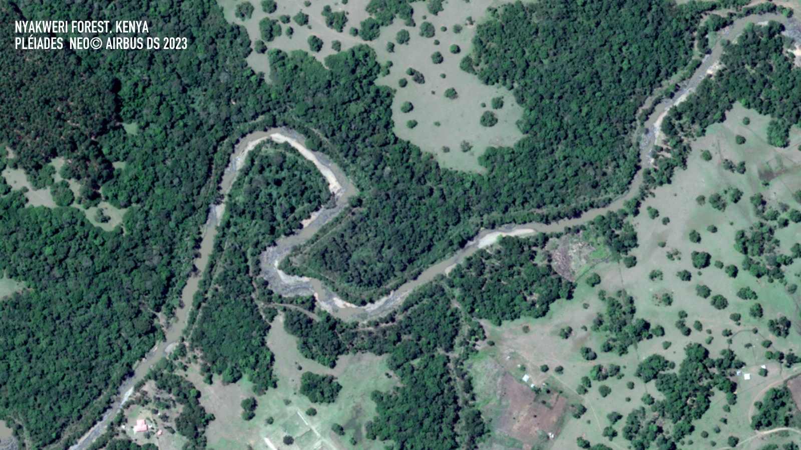
- Nyakweri Forest, a critical habitat in Kenya's Greater Mara Ecosystem and the newly identified eastern range of the giant pangolin faces significant threats from deforestation, fragmentation, electric fences and poaching.
- This study employed AI and 30 cm VHR satellite imagery from Pléiades Neo to assess habitat degradation and inform conservation strategies for this ecosystem.
- A deep learning model was developed to detect key landscape features, such as forest cover, roads, water sources and fences, to help target conservation initiatives like wildlife corridors, fence de-electrocution and restoration efforts.
- Each year, an estimated 1,000 to 2,000 pangolins die in South Africa alone from electrocution after instinctively curling around electric fences in a defensive response—fences that were designed to protect them. The number of deaths in Africa more widely is unknown.
- This study developed a specialised fence detection model using 65,000 fence examples. This model assisted field teams in mapping fences and informed community engagement and efforts to mitigate electrocution risks.
- Part 2 of this study analysed deforestation trends to map remaining forest cover, identified key deforestation drivers and pinpointed priority areas for habitat restoration.
Objectives
Introduction
Nyakweri Forest, located in Kenya's Greater Mara Ecosystem, is a crucial Afromontane forest habitat, vital for maintaining biodiversity and ecosystem services. It has gained significant recent conservation attention due to its ecological importance and the threats it faces. In 2022, The Pangolin Project made a groundbreaking discovery that dramatically altered our understanding of giant pangolin distribution in East Africa.
Giant pangolins (Smutsia gigantea), the largest pangolin species, were once thought to range only as far east as Uganda. However, research by The Pangolin Project confirmed their presence in Nyakweri Forest, extending their known range 500 km eastward. This discovery not only underscores the forest's ecological value but also highlights its critical role in pangolin conservation.
Unfortunately, Nyakweri Forest is also at high risk. Over the past decade, more than half of its forest cover has been lost due to habitat destruction and fragmentation, primarily driven by conversion to farmland. This ongoing degradation is causing irreversible damage to the ecosystem, threatening both the forest’s biodiversity and its ability to support species like the giant pangolin.
The key threats to Nyakweri Forest and its Giant Pangolin population are:
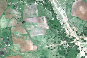
Deforestation: Large-scale clearing of forest for agriculture, charcoal production and human settlement. Giant pangolins prefer dense forest habitats with abundant populations of ants and termites.
Habitat fragmentation: The remaining forest is increasingly divided into smaller, isolated patches. The construction of field boundaries, roads and buildings further encroaches on natural habitats and destroys the connectivity between “islands” of remaining viable habitats.
Electric fences: While intended to protect crops from elephants and other raiding species, these pose a significant physical threat to pangolins, causing death from electrocution.
Poaching: All pangolin species are highly valued for their meat and scales. Pangolins are the most trafficked wild mammal globally.
Methodology
The project aimed to develop a low-code deep learning workflow to rapidly assess habitat degradation across 1,000 km², including land partitions, buildings and tree cover. Designed for accessibility, it aimed to enable ecosystem connectivity assessments and other conservation challenges, making advanced technology available to projects with limited resources.
Data
|
Number of images |
Date of capture |
Description |
Coverage |
|
3 |
24/08/2023 |
4-band pan-sharpened product consisting of 3 RGB (Red, Green, Blue) bands and 1 NIR (Near-Infrared) band with a resolution of 0.3m |
450km² |
|
2 |
02/10/2023 |
500km² |
|
|
1 |
01/03/2024 |
130km² |
Table 1: Data description. The project utilised Airbus Pléiades Neo imagery
|
Imagery Examples |
||
 |
 |
 |
|
Tranche 1 |
Tranche 2 |
Tranche 3 |
Table 2: Examples of imagery
Data preprocessing
A single band Normalised Difference Vegetation Index (NDVI) version of the merged data was created and overlayed on the RGB image to enhance features and assist during manual digitisation.
Hardware
The project utilised a desktop computer with the following hardware specifications:
- Processor: 13th Gen Intel(R) Core (TM) i5-13600K, 3.50 GHz
- Memory: 64GB Corsair Dominator Platinum DDR4 6600 MT/s
- Storage: Samsung 990 Pro 4TB NVME SSD
- Graphics Processing Unit: NVIDIA GeForce RTX 4090 24GB GDDR6
The project's computing infrastructure selection process carefully weighed the relative merits of cloud versus local computing solutions. Local computing infrastructure offered several compelling advantages for this implementation. The local environment significantly simplified the workflow by maintaining all processes in a single environment, eliminating data transfer overhead and providing predictable costs and performance characteristics. Moreover, the hardware requirements for general data handling, preprocessing, and analysis would have necessitated substantial local computing resources regardless of the chosen compute strategy.
For a scalable approach capable of processing much larger areas, or regularly iterating over time series data, a cloud solution would likely represent a logical progression.
For software, the project used ArcGIS Pro.
Deep learning model
The selection of an appropriate computer vision approach required careful consideration of various methodologies within the field. Image classification, while effective for categorising entire images, provides limited spatial information and wouldn't capture the detailed landscape features needed for this analysis. Semantic segmentation offers pixel-level classification and was seriously considered a viable approach. It would have provided precise delineation of features and potentially superior handling of complex boundaries. However, the object detection approach was ultimately selected because it better aligned with the project's analytical goals.
The key advantage of object detection for this implementation was its ability to treat landscape features as discrete entities rather than pixel classifications. This approach naturally facilitates quantitative analysis - counting buildings, measuring fence lengths, and analysing feature relationships become more straightforward when working with bounded objects rather than pixel masks. Object detection also provides an inherent framework for confidence scoring at the feature level, allowing for more nuanced filtering and post-processing of results. The polygon-based output format integrates seamlessly with GIS workflows, enabling direct spatial analysis without the need to convert pixelwise classifications into vector features.
Within the object detection framework, the ResNet architecture was selected, initially implementing ResNet-152 before transitioning to ResNext-101 for the final model. This choice balanced sophisticated feature learning capabilities with practical resource requirements, enabling effective model training and deployment while maintaining robust detection performance.
Training data preparation
Approximately 7.5% of the total imagery provided was labelled for training. This was distributed across 7 sample areas, totalling about 78km² across the three imagery tranches. These areas were manually selected for a high density and diversity in the desired classes, as well as having a high level of representation of the various locale types found within the target geography.
All image chips and labels were resized to 224x224 pixels which is the size required by the backbone model architecture and then exported using the "Export Training Data for Deep Learning" tool within ArcGIS Pro for model training.
Model training
Data augmentation
To improve performance and generalisation, several data augmentation techniques were applied. A 180-degree rotation helped the model adapt to lighting and shadows, while five random augmentations—zoom, crop, brightness, rotation and saturation—expanded each image into 11 variations.
The model trained for 20 epochs with a batch size of 16, using a dynamically optimised learning rate. A 20% overlap stride ensured sufficient feature representation across image chips.
Figure 1: Training data generation

Results
Model performance iteration
Iteration 1 - Table 3: Initial 7-Class Model Classification Performance
|
Class |
Accuracy |
Class |
Accuracy |
|
Vegetation |
50.7% |
Clouds |
55.8% |
|
Buildings |
71.6% |
Fencelines |
4% |
|
Partitions |
16% |
Water bodies |
23.3% |
|
Roads |
27% |
|
|
Model precision scores varied by feature type. Buildings (71.6% precision) and vegetation (50.7%) had clear geometric signatures, allowing accurate boundary delineation. Due to Intersection over Union limitations (IoU), linear features like roads and fences had lower precision (27% and 4%, respectively). Since these features are often just a few pixels wide, minor spatial offsets significantly reduced scores despite correct identification.
Fence detection was particularly challenging, as feature width often fell below image resolution. To address this challenge, we developed a specialised fence detection model trained on an expanded dataset of 65,000 fence examples. This dedicated model, optimised specifically for linear feature detection, improved precision from 4% to 16%. While this improvement might appear modest in absolute terms, it represented a significant enhancement in practical utility, particularly in identifying fence networks and their distribution across the landscape when operating at lower confidence thresholds between 20-30%.
Fenceline detection
|
Comparison between raw imagery and successive fence detection models |
||
|
a) |
b) |
c) |
|
Manually drawn fences |
General model (4% precision) |
Dedicated model (16% precision) |


Figure 2: Showing (a) Raw imagery, (b) result from the general model at 4% precision and (c) result from the dedicated model at 16% precision
The disconnect between precision scores and practical utility stems from detection methods. For example, a fence detection model may correctly locate a fence but generate a slightly wider bounding polygon to capture contextual features. This lowers IoU scores but improves reliability by distinguishing fences from similar elements like tracks or field edges.
To address this, confidence thresholds were calibrated by feature type, from 65% for vegetation to 22% for fences, balancing sensitivity and false positives. While not ideal for precise mapping, this approach effectively supported landscape analysis and conservation planning by identifying feature densities and distributions.
These findings highlight that strict precision metrics don’t always reflect practical utility. Even models with modest precision scores can provide valuable insights when interpreted within the right context.
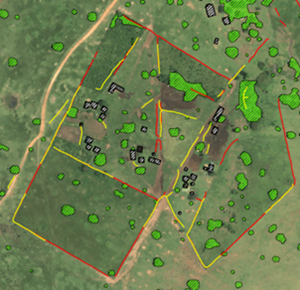
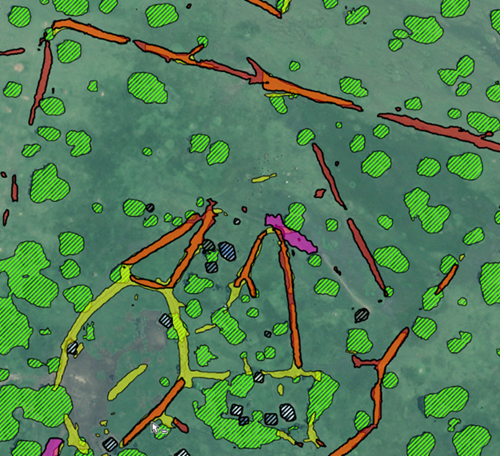
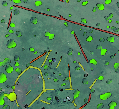
Linear partitions detection
|
Example output of linear features |
|
 |
 |
|
Raw imagery |
Detected partitions (yellow) and fences (red) |
Figure 3: Showing (left) raw imagery and (right) detected partitions and fences

Figure 4: Showing manually digitised fence lines (red) overlaid on forest patches (green)
Analysis of fencing
The first iterations of the model, as well as the final 7-class model, had poor performance for fences, necessitating a bespoke fence-specific model with a greatly expanded training dataset for this class.
Due to the difficulty of accurately mapping fences using the model, the model was used primarily for general fence detection, rather than production mapping of the features themselves. Once the fences were detected, they would be hand-drawn within the Priority Conservation Area (PCA) and surrounding area to create a comprehensive map of fence lines. This had the added advantage of generating high-quality training data that will be used to train successive versions of the model.
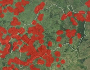
Whilst this does not indicate whether the fences are electrified, it provides a useful starting point to identify priority areas for ground verification and community engagement. To achieve this fence lines within 100m of remaining forest were filtered. From here nearby homesteads near those fence networks were grouped into communities and highlighted for engagement. Most such communities lie within the western area of the PCA, which is has the highest concentration of fences.
|
Fences within 100 m of forest filtered |
Fencing areas buffered to 200 m |
 |
 |
|
Communities within 200 m of a fence identified |
Example of identified communities/homesteads |
 |
 |
Figure 5: Showing fences within 100 m of forest (top left), 200 m buffer around fences (top right), households within 200 m from fences (bottom left), and a closer view of the households relative to the fence lines (bottom right)
Post-processing
All features under 5 m² were removed to eliminate small misdetections. Buildings were regularised for clearer shapes, improving geometry, though complex forms remain imperfect.
A process was also derived to convert the linear feature polygons to line features. This included the generalisation of polygons to capture their general direction and remove irregularities, collapsing capturing centrelines using the collapse polygons tool and deleting short segments to improve the output. Many output features are larger than the 224x224 pixel processing size however the model produced output polygons no larger than 224x224 pixels in size. This left many larger objects comprised of several constituent output polygons. To smooth output, a degree of overlap was maintained.
However, to achieve clean output polygons of the feature classes, objects were dissolved by class so overlapping features formed one feature class. A summarise within process was then applied across the dissolved features and the constituent features to establish the mean confidence of the constituent polygons. This was weighted by the proportion of the summarised constituent layer within the dissolved polygons and grouped by class.
|
Building regularisation |
|
 |
 |
| Before regularisation | After regularisation |
Figure 6: Showing post-processing of building features before regularisation (left) and after regularisation (right)
|
Comparison between raw output and dissolved features |
|
 |
 |
| Raw output features | Dissolved features |
Figure 7: Showing post-processing by dissolving to remove overlapping features
Test Time Augmentation
Test Time Augmentation (TTA) improves model accuracy by applying flips and rotations to input images, running multiple inferences and averaging results. Outputs below the 50% confidence threshold for the PCA were discarded. TTA enhanced boundary accuracy, reduced detection sprawl and minimised false positives, but sometimes removed smaller or lower-confidence detections.
Due to high computational costs, TTA was applied only to the 130 km² PCA at 50% confidence, while the larger 1018 km² area used a 25% threshold without TTA. A more efficient approach would involve running inference at 15% confidence and filtering out low-quality detections before merging results.
|
Comparison of output using TTA |
|
 |
 |
| Comparison of output using TTA | With TTA |
Figure 8: Showing comparison without (left) and with Test Time Augmentation (right)
|
Example output Using TTA |
|
 |
 |
| Raw imagery | Detection of wire fence using TTA |
Figure 9: Showing an example of output using Test-Time Augmentation
Conclusion
This project has demonstrated the power of AI and high-resolution satellite imagery in quantifying habitat degradation and informing conservation strategies. While the model performed well in identifying broad landscape features, challenges remain in detecting linear elements such as fences and roads. Refining a dedicated fence detection model improved accuracy, but further work is needed to enhance precision and scalability.
The next phase will test the model in areas beyond Nyakweri Forest to assess its adaptability and improve robustness with new training data. A bespoke forest cover model using NICFI 5m data will enhance deforestation and habitat monitoring. Cloud-based infrastructure will be adopted for faster processing and expanded conservation planning, such as highlighting potential corridors where buffers intersect.
Interactive dashboards will make AI-driven insights accessible to conservationists and policymakers. Layering this analysis with other datasets will improve the understanding of habitat connectivity and threats, guiding reforestation efforts, particularly for the Giant Pangolin. Experimenting with multispectral views will refine feature detection and highlight priority areas for community engagement. Though not a standalone tool, this AI-driven workflow offers a scalable approach to guide conservation strategies. With ongoing refinement, it can support Nyakweri Forest protection and broader ecosystem conservation.
Langland Conservation
Project Lead
Ruari Bradburn
Langland Conservation is a UK-registered charity that specialises in using data analytics and technology to support a range of conservation partners.
Their work focuses on using data-driven insights to help decision-makers achieve greater results in conservation, empowering others to leverage technology in conservation efforts and supporting investigations to tackle organised wildlife crime worldwide.